Exploring results
Once complete, we make your simulation results available in several different – via an interactive results page, as a printable PDF report, an Excel spreadsheet & as raw VTK data (for local/custom post-processing).
We also have a growing number of comparison tools within AeroCloud which are discussed in the following section.
Here is a summary of each of the main ways you can explore your results.
Interactive results page
Each simulation has its own interactive webpage where you can explore and analyse its results in detail.
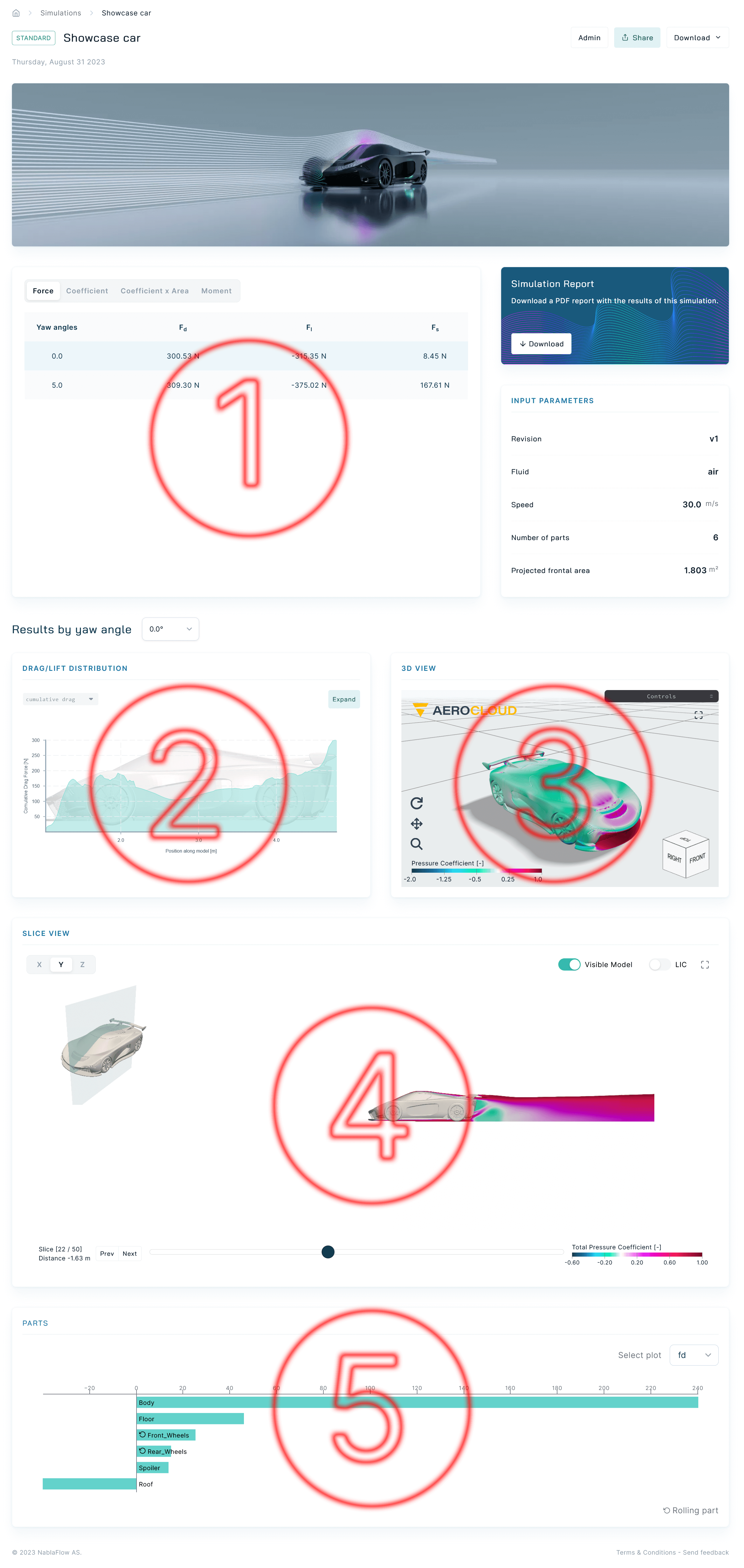
1: The table panel
This panel shows the total forces acting on your model at each yaw angle (including presentation in coefficient form) and the moments about the model origin.
The yaw angle toggle (immediately below the table panel) can be used to select which yaw angle is shown in the subsequent panels.
2: The force distribution panel
This panel plots the distribution of forces across your model. The technique effectively slices your model into a number of segments & reports the forces acting on those segments.
Use the dropdown menu to switch the chart between lift, drag & side force in the X, Y & Z directions to show the force acting on each of the model segments.
The raw force data on these segments can be noisy, so we smooth the data slightly to produce a more readable plot. We also normalise the data by the width of the segment to allow easier comparison across models of different lengths.
Alternatively, you can choose to show cumulative lift, drag & side force distributions, where the raw segment forces are summed along the length of the model (always in the X-direction).
The cumulative force plots are particularly useful for quickly identifying where force changes occur along the length of your model.
Check out the multi-run, comparison version of this plot to quickly compare the force distribution across multiple runs from your project.
3: The 3D-view
This panel loads an interactive 3D model which can rotated & zoomed to get the perfect view of your model surfaces.
Models are loaded on request (to speed up page load) click to activate this panel.
By default your model will be coloured by surface pressure, but you can also choose to colour by skin friction, drag pressure or heat transfer - click on the controls panel & use the model dropdown menu to make your selection.
You can use the control panel to toggle pressure contours (isosurfaces which illustrate the shape of the wake around your model) and streamlines. The orientation & position of the streamlines can be changed interactively using their own dropdown & slider bar.
If your model contains multiple parts then you can optionally hide individual parts from view. Hover your mouse over the part you want to hide & right-click to bring up the option.
Right-click anywhere in the window to bring up the option to show all of your parts again.
The 3D view panel can also be expanded to fullscreen using the buttons on the right-hand side of an active panel (excellent for detailed screenshots).
Click the “?” for a short tour of the 3D view.
4: The slices view
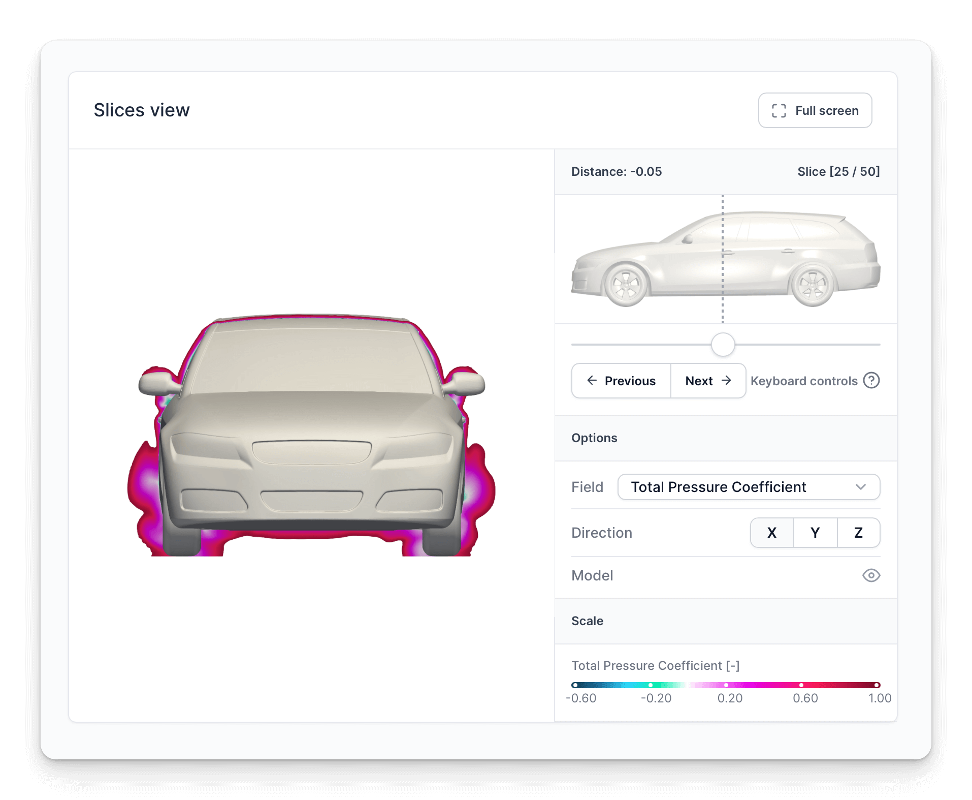
The slices view gives you an insight into what is going on in the flow around your model, using contours plotted on planar slices, which can be swept along the primary axes.
The left panel shows the results, with the controls on the right.
At the top you have an indication of where the currently displayed slice is in relation to your model. Move the slice using the slider, previous & next buttons or even the left/right arrow keys.
There are several fields available to view, including total pressure coefficient, static pressure coefficient & acoustic power.
You also have the option to view the total pressure slices with LIC pathlines (a technique similar to oilflow or streamlines, which reveals the in-plane flow structures that are present in your data).
Slices are available in X,Y & Z directions & can be viewed with & without the 3D model. These features can be accessed via the control panel on the right, or via the X, Y, Z & M keyboard shortcuts respectively.
The slice viewer panel can be expanded to full screen using the button in its top right corner (excellent for checking out the detail in the LIC data).
5: The parts panel
This bar chart shows the forces and moments acting on each individual part of your model, along with heat transfer and surface area per part.
Hover your mouse pointer over the bars to see the numeric value for each part.
Use the dropdown menu to select the component of interest:
- $F_d$ = Drag Force (Force in the X-Direction) $[N]$
- $F_s$ = Side Force (Force in the Y-Direction) $[N]$
- $F_l$ = Lift Force (Force in the Z-Direction) $[N]$
- $M_r$ = Roll Moment (Moment about the X-Axis) $[Nm]$
- $M_p$ = Pitch Moment (Moment about the Y-Axis) $[Nm]$
- $M_y$ = Yaw Moment (Moment about the Z-Axis) $[Nm]$
- Total convective heat transfer rate per $\Delta T$ $[{W \over K}]$
- Averaged heat transfer coefficient $[{W \over {m^2 K}}]$
- Wetted surface area $[m^2]$
Printable PDF Report
A printable report (in PDF-format) can be downloaded from the main results web page.
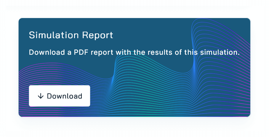
This report contains additional information (not shown on the web page) including simulation-specific settings, plus definitions and explanation of the result parameters.
It also includes a detailed summary of your simulation data via a wide selection of plots, tables and charts.
Example report
Download an example report here.
Excel Spreadsheet
Numerical data (e.g. forces, moments & heat transfer) are available in a single .xlsx spreadsheet format.
The spreadsheet includes data for each of your model parts, at each yaw angle & can be used as a record or to construct your own comparison tables.
The spreadsheet also includes data for the force distributions, should you wish to plot your own charts.
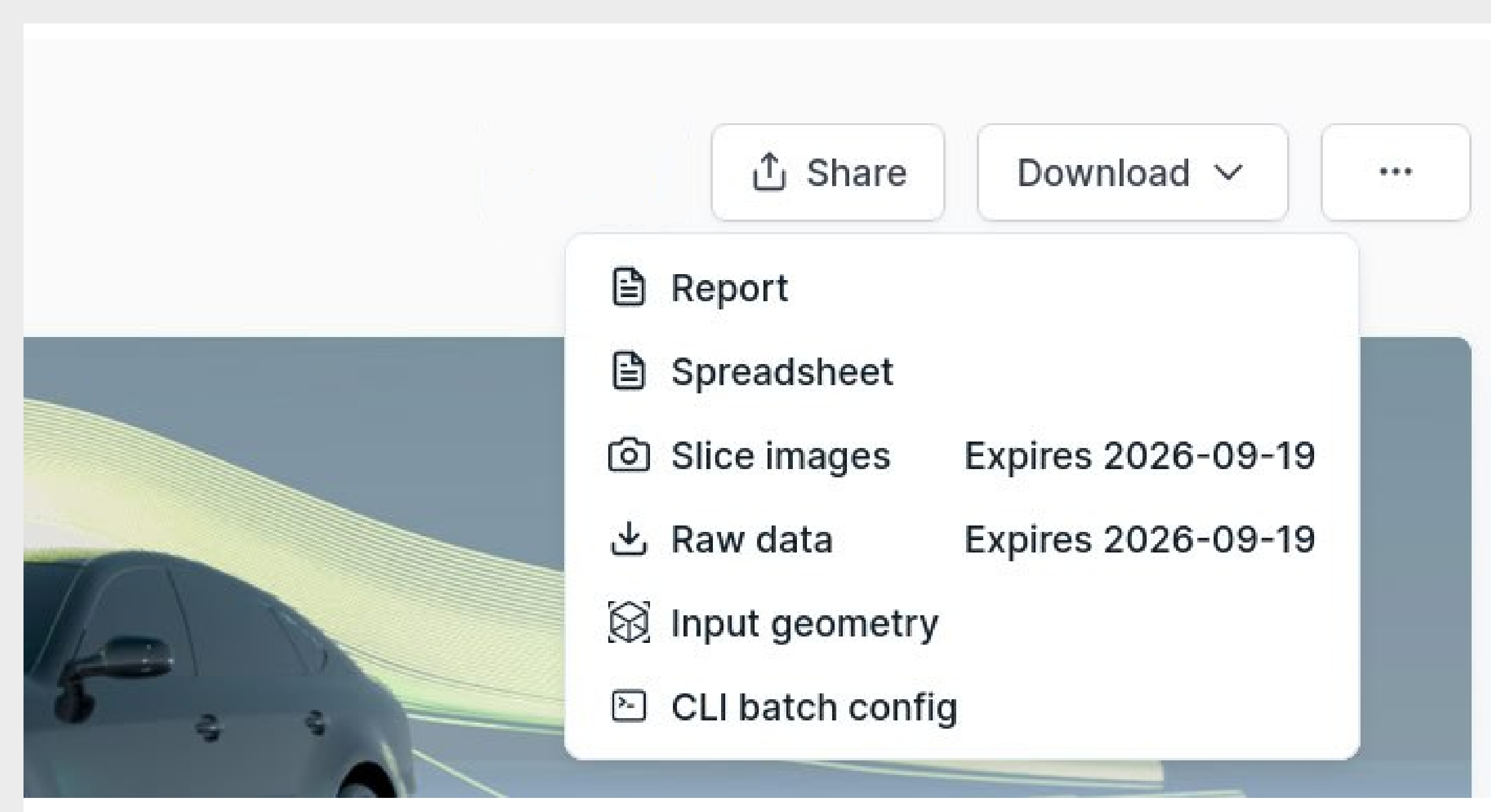
The spreadsheet can be downloaded via the dropdown menu at the top of your simulation webpage.
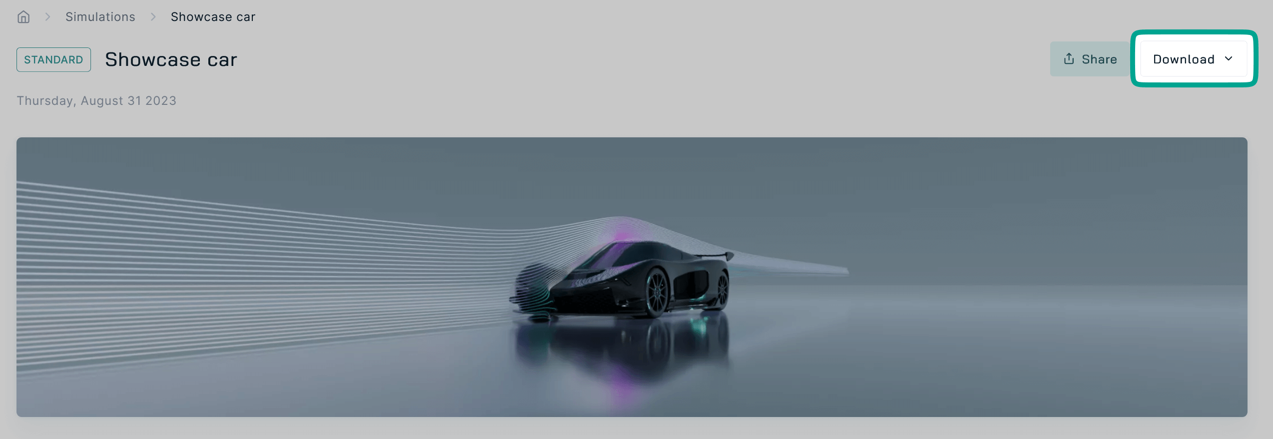
Raw Data
The raw CFD data can be downloaded to your local machine where you can perform your own custom post-processing, analysis and visualization.
The data is provided in VTK format, which can be read using the free, open-source visualisation tool, ParaView (& many other tools).
Access the raw data download link via the dropdown menu at the top of your simulation results page.
The raw data files are large (10GB+ for Pro simulations) & are therefore only available for a limited time (60 days) after the simulation is finished.
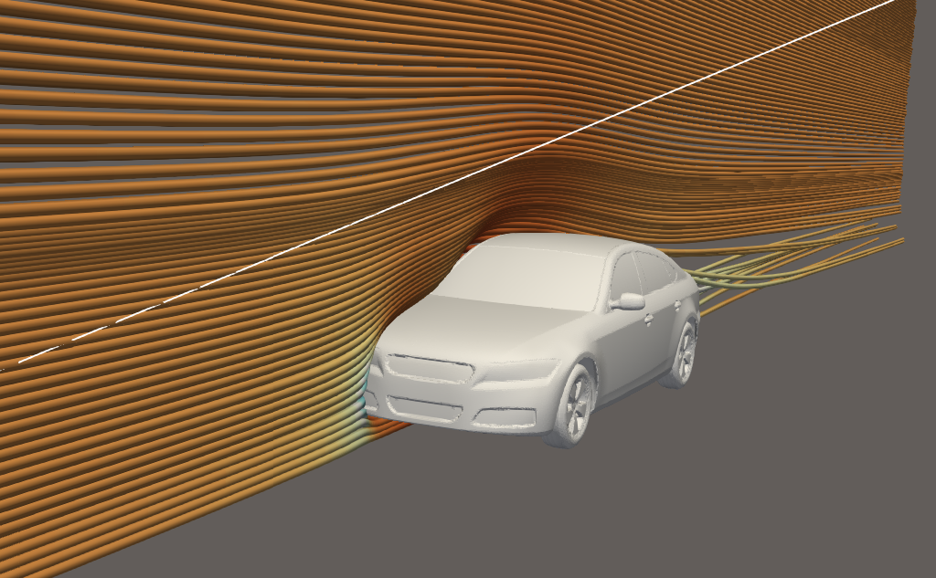
To perform a deeper flow analysis with higher streamlines density, the following procedure can be exploited:
- Download Raw Data. Begin by downloading the raw data from the website.
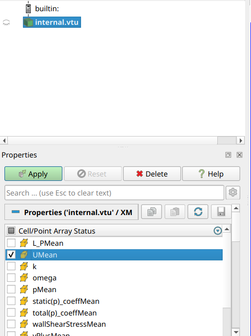
- Load Internal Data. In ParaView, load the internal.vtu file. Deselect all cell point arrays, except for UMean.
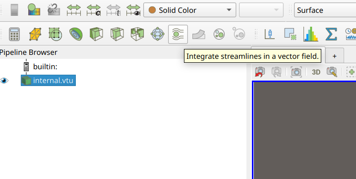
- Apply StreamTracer Filter. Apply the StreamTracer filter to visualize streamlines.
Add Tube Filter. Press Ctrl + Space to search for the Tube filter and apply it.
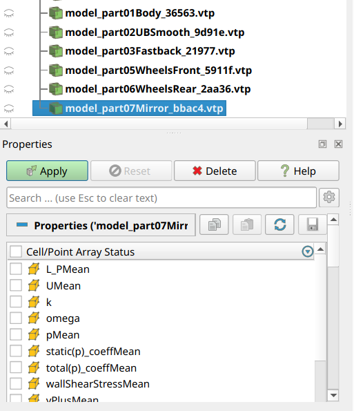
Load Boundary Data. Load all .vtp files from the boundary folder. Deselect all cell arrays, then apply the settings.
- Adjust Streamline Points. Select StreamTracer1 in the Pipeline Browser. Scroll down to find this section:
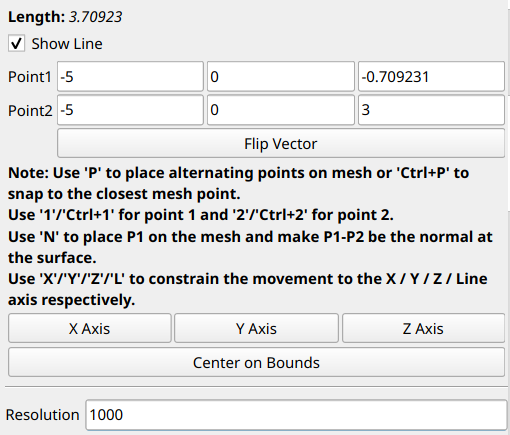
Here, you can specify the origin and endpoint of the streamlines source. Alternatively, select an axis (e.g., Z-axis), adjusts X coordinate to place the source in front of the model and adjust the Z coordinate to include the model and avoid extending too far into the free stream. Apply these settings.
- Adjust Resolution. Below the points section, modify the Resolution to control the number of streamlines to display. Apply the changes.

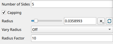
- Refine Tube Visualization. Select Tube1 in the Pipeline Browser. Reduce the number of sides to decrease computational load. Adjust the Radius slider to improve visualization clarity.
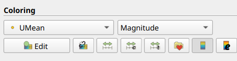
- Color Streamlines by Wind Speed. In the Coloring sub-menu, select UMean to color the streamlines based on wind speed, providing a visual interpretation.
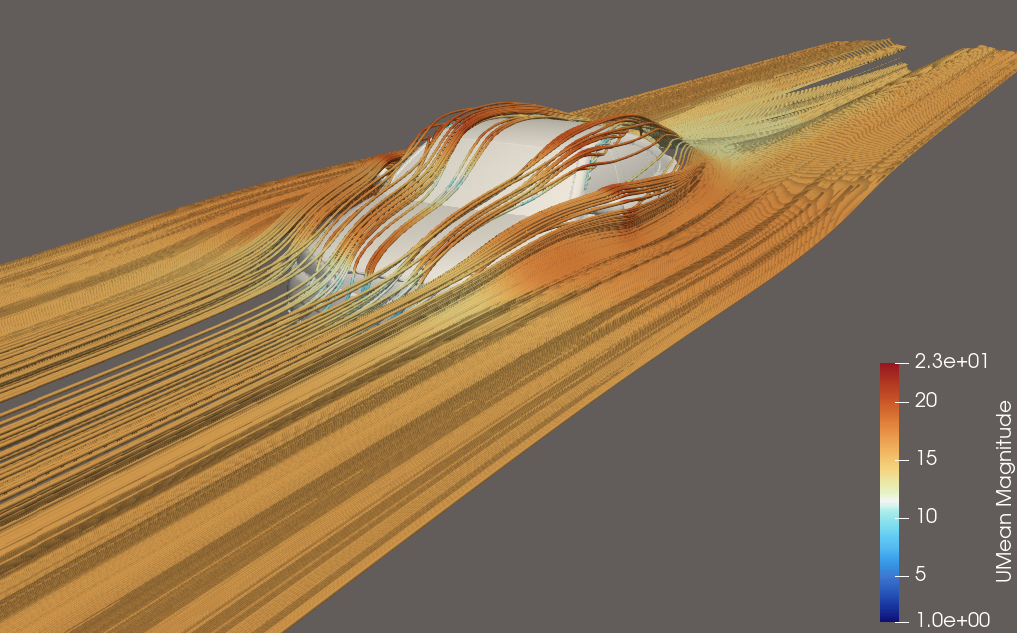
Outcome:
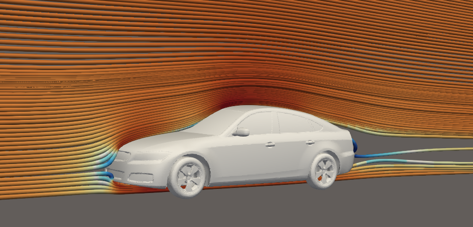
Adjusting the number of streamlines, tube radius, and number of sides will help you refine the visualization resolution. Additionally, shifting the Y-coordinate moves the streamlines along the model:
Changing the constraint axis allows for different views:
More details about our simulation data expiration policy can be found here.