Simulating Trees

Why Simulate Trees?

Trees not only convert carbon dioxide into oxygen and eliminate pollution and airborne toxins, but they also significantly influence wind patterns as it passes through their leaves. Trees play a crucial role in enhancing pedestrian wind comfort in urban areas. Here are the key points:

1. Windbreak Effect: Trees act as natural windbreaks, reducing wind speeds at ground level. Even a single tree can make a noticeable difference, creating a more comfortable environment for pedestrians. Removing all trees from an area can double the wind speeds, significantly decreasing pedestrian comfort.
2. Canopy Density and Shape: The shape and density of tree canopies are important. Denser canopies with lower porosity provide better wind sheltering.
3. Aspect Ratio: The aspect ratio (height to width ratio) of a tree canopy affects the size of the sheltered zone behind the tree and the distance required for wind speeds to recover.
4. Bare Branches in Winter: Even the bare branches of deciduous trees in winter can moderate airflow and reduce wind pressure on buildings.
5. Sheltering Effect Distance: The sheltering effect of trees extends up to around seven times their height downwind, with the most significant reduction in wind speed occurring within 0.5 times the tree height.

Urban planners and designers should consider tree planting and species selection to maximize pedestrian wind comfort. Strategic placement of trees can serve as effective windbreaks, significantly enhancing outdoor spaces.

Different tree species, characterized by varying shapes, sizes, and leaf types, affect wind velocity to different extents. While wind is not completely stopped by trees, its speed is reduced as it moves through their branches. The key factor here is leaf density: trees with denser foliage offer greater resistance to airflow. For instance, a Silver Birch tree has less air resistance compared to a Chestnut tree due to its lower leaf density.

This ability of trees to allow air to pass through is known as porosity and is quantified using a leaf area index (LAI). The LAI values are determined through experiments.

When trees with high leaf area index values—indicating greater wind resistance—are strategically placed in areas with fast airflow and strong winds, they can significantly improve wind comfort and safety for pedestrians. These trees act as effective windbreaks, creating more pleasant and secure outdoor environments. For more detailed explanations on this topic, refer to the upcoming webinar.

How Do You Simulate a Tree?

Introduction

In Computational Fluid Dynamics (CFD), trees can be modeled as porous media to accurately represent their impact on airflow. This approach considers trees as objects that allow air to pass through while imposing resistance, thus affecting wind speed and turbulence. Modeling trees as porous media is essential for understanding environmental phenomena like windbreaks, pollution dispersion, and microclimate regulation.

Concept of Porous Media

Porous media are materials containing pores (voids). The flow through porous media is characterized by the interaction between the fluid and the solid matrix. In the context of trees:

• The foliage and branches constitute the solid matrix.
• The spaces between leaves and branches act as the pores through which air flows.

Key Parameters in Porous Media Modeling

To represent the plant canopy regions, the user must specify the C_d and LAD values.

1. Leaf Area Density (LAD):
   • Definition: LAD is the leaf area per unit volume of foliage.
   • Role: Determines the porosity of the tree and influences how much air resistance the foliage provides.

LAD is a local characteristic, it is common to make the hypothesis of horizontal homogeneity. However, LAD will depend on the vertical location LAD(z). The empirical relation allows us to link LAD(z) to a global quantity LAI. The values for LAI can be found in the literature.

LAI Values for Woody Plants

$$ LAD = LAI * \frac{h_t - z_m}{h_t - z}^n \exp {n{ 1 - \frac{h_t - z_m}{h_t - z}}} $$

Here are some of the values for the most common species of trees in Europe:

2. Drag Coefficient C_d:
   • Definition: A dimensionless number representing the drag force exerted by the leaves and branches.
   • Role: Used in momentum equations to calculate the resistance offered by the tree to the airflow.

Equations for Modeling Trees as Porous Media

We base our tree model on the OpenFoam atmPlantCanopy sources. To apply the atmPlantCanopy sources, the user must specify the C_d and LAD values in the constant/fvOptions file for the desired cell zones representing the plant canopy regions.

We provide the relation that supposes the foliage density is independent of the vertical direction. This is a simplification to generalize the LAD at the volume of the tree with an average value:

$$ LAD = \frac{LAI}{h} $$

1. Momentum Sink Term:

   Represents the loss of momentum due to the drag force of the tree.

   $$ S_p = - \alpha \rho C_d LAD |u_0| u $$

   Where:

   • S_p is the source term applied to the momentum equation
   • α is the phase fraction (1 for single-phase flows)
   • ρ is the fluid density
   • C_d is the plant canopy drag coefficient (a user-specified value)
   • LAD is the leaf area density (a user-specified value representing the plant canopy density)
   • |u_0| is the magnitude of the velocity field from the previous iteration
   • u is the current velocity field

The source term S_p acts as a drag force opposing the flow velocity u within the plant canopy region. The magnitude of this drag force is proportional to the leaf area density LAD and the drag coefficient C_d, which characterize the plant canopy geometry and aerodynamic properties.

This source term is then incorporated into the momentum equation during the solution process, effectively reducing the velocity within the plant canopy regions to account for the drag induced by the vegetation.

2. Turbulence Source Term:

For the turbulence kinetic energy dissipation rate (\epsilon) equation:

$$ S_p = \alpha \rho \left( C_1 - C_2 \right) C_{\text{canopy}} \epsilon $$

with:

$$ C_{canopy} = 12.0 \sqrt{C_\mu} C_d LAD |u_0| $$

Where:

• S_p = Source term without boundary conditions
• C_1 = Model constant (epsilon-based models) [-]
• C_2 = Model constant (epsilon-based models) [-]
• C_\mu = Empirical model constant [-]
• \epsilon = Turbulent kinetic energy dissipation rate (Current iteration) [m²/s³]
• C_d = Plant canopy drag coefficient [-]
• LAD = Leaf area density [1/m]
• |u_0| = Previous-iteration velocity field [m/s]
• C_{canopy} = Plant canopy term
• \alpha = Phase fraction in multiphase computations, otherwise equals 1
• \rho = Fluid density in compressible computations, otherwise equals 1

The source terms S_p account for the production and dissipation of turbulence within the plant canopy region. The magnitudes of these source terms are proportional to the leaf area density LAD and the drag coefficient C_d, which characterize the plant canopy geometry and aerodynamic properties.

These source terms are then incorporated into the turbulence transport equations during the solution process, effectively modifying the turbulence levels within the plant canopy regions to account for the effects of vegetation.

How to Upload Your Tree 3D Model?

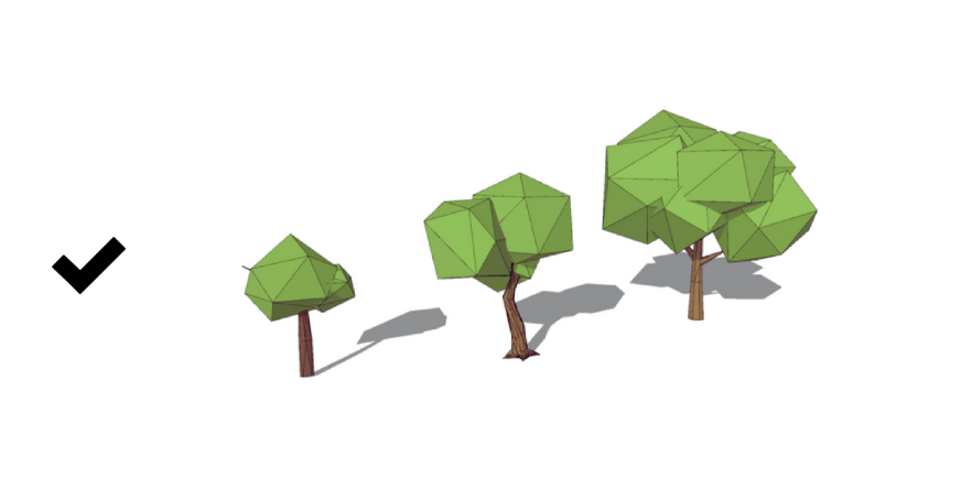
ArchiWind allows adding vegetation under the Trees patch. Trees are a key agent for mitigating wind exposure locally. They will act as a porous medium and naturally dissipate excessive wind energy. The optimal placement for trees can be assessed through the comparison feature. Tree geometries are to be expressed as volumetric shapes. Adding trees with foliage represented as surfaces or aggregating tiny elements will not be recognized properly.